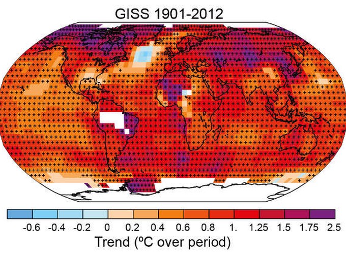
In this map building tutorial we’ll focus on the issue of combining high fidelity vector graphics with coarse resolution raster data. When combining both vector graphics (lines / polygons) with raster data a discrepancy in resolution between the two can lead to a staircase effect in rendered edges. You can easily see how this issue can arise when trying to fit coarse resolution data, such as the Goddard Institute for Space Studies (GISS) global temperature analysis data, into country polygons to display only the land surface trend. Below we discuss, and provide worked examples, how to solve these resolution issues.
Fixing coarse resolution raster issues
A basic map
As in the first tutorial we begin building the map with loading some essential libraries. In addition, we create some fake data coarse resolution raster data for illustration purposes. The fake raster data covers both land and oceans around Europe. If you overlay this raster map with country polygons you clearly see a resolution mismatch.
In some cases visualizing data as such isn’t an issue. However, in other cases you might want to emphasize either the land or ocean component of your raster dataset. Another scenario arises when the raster data is either land or ocean based, but still at a coarser resolution then the vector outlines you want to map these data with. In all these cases, a mismatch in resolution between data sources will be visible in your final rendered map.
Note that in this example we’ll use the most basic plotting style as the aim is to illustrate various techniques, and not focus on the overal aesthetics! Various styling elements will be covered in other blog posts.
# load libraries
library(raster)
library(tidyverse)
library(rnaturalearth)

# grab country outlines / ocean areas as sf object
countries <- ne_countries(returnclass = "sf", scale = 50)

# create a fake coarse grid raster
# with a "EU" extent
r <- matrix(rnorm(100),10,10)
r <- raster(r)
extent(r) <- c(-20,20,30,70)

# convert raster to dataframe
# for ggplot2 plotting
r_df <- r %>%
  rasterToPoints %>%
  as.data.frame() %>%
  filter(layer!=0)

p <- ggplot() +
  geom_raster(data = r_df,
            aes(x = x,
                y = y,
                fill = layer)) +
  scale_fill_continuous() +

  geom_sf(data = countries,
          color = "white",
          fill = NA,
          size = 0.2) +

  # crop
  coord_sf(xlim = c(-20, 20),
           ylim = c(30, 70))

print(p)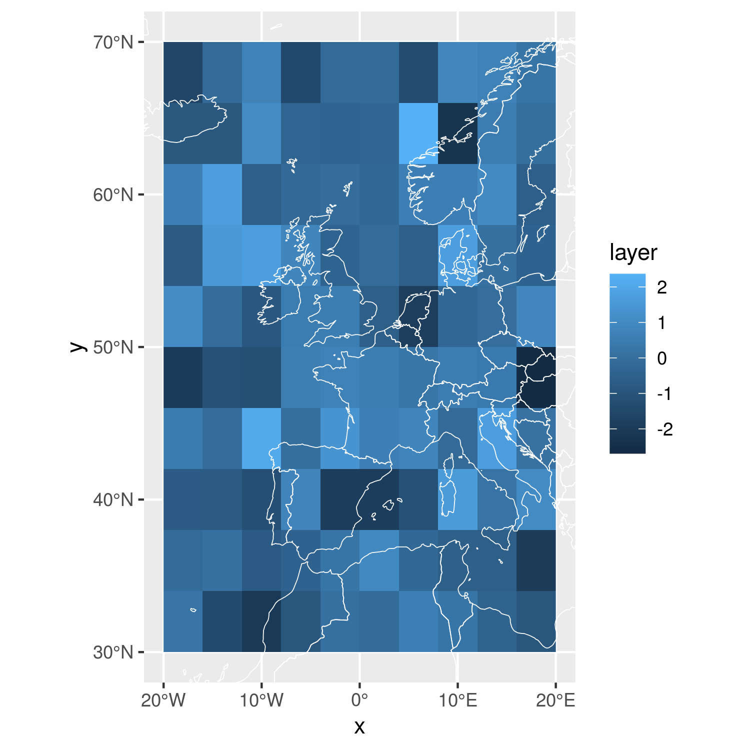
The intuitive approach would be to mask out the raster data using the vector polygon used. Depending on the algorithm used more or less pixels will be included. Yet, the end results remains undesirable and leaves very rough edges around polygons. In a slightly higher resolution image it would give sawtooth edges to the plot.
# mask these values using the countries
# and convert to dataframe for ggplot2
# plotting
r_m <- mask(r, countries)
r_m_df <- r_m %>%
  rasterToPoints %>%
  as.data.frame() %>%
  filter(layer!=0)


p <- ggplot() +
  geom_raster(data = r_m_df,
            aes(x = x,
                y = y,
                fill = layer)) +
  scale_fill_continuous() +

  geom_sf(data = countries,
          color = "white",
          fill = NA,
          size = 0.2) +

  # crop
  coord_sf(xlim = c(-20, 20),
           ylim = c(30, 70))

print(p)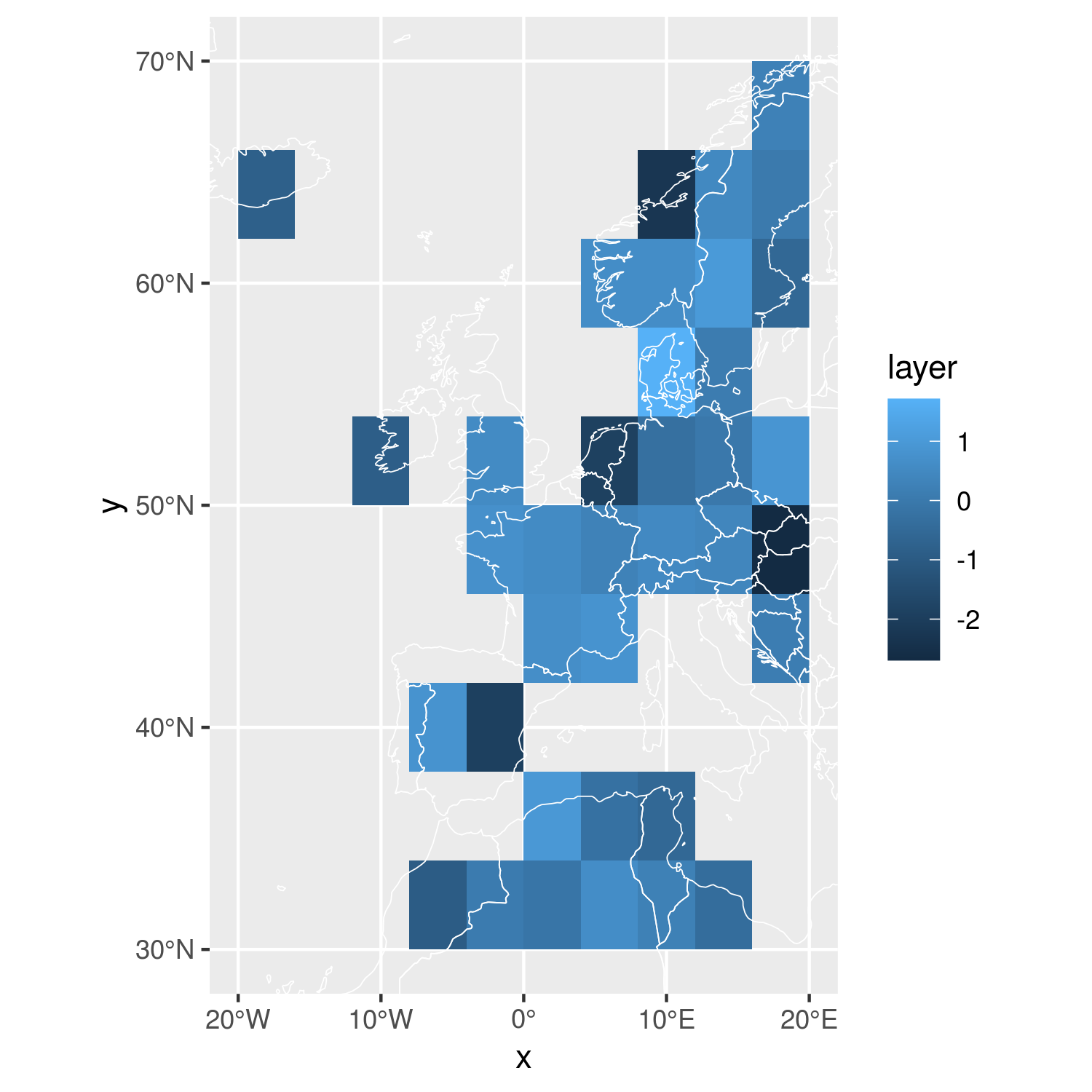
The tricks
cover it up
The easiest way to hide this resolution mismatches is do just that. You can cover up the undesired areas using a polygon with the same colour as the background of the plot! This methods is fast but depends on the components in your plot you still want to render. Depending on the complexity of your plot you might run into trouble with this method, overplotting data you still want to show.
# THE COVER UP
# download ocean outlines
ocean <- ne_download(
  scale = 50,
  type = "ocean",
  category = "physical",
  returnclass = "sf")

# overplot the undesired coarse raster edges
p <- ggplot() +
  geom_raster(data = r_df,
              aes(x = x,
                  y = y,
                  fill = layer)) +
  scale_fill_continuous() +

  geom_sf(data = ocean,
          color = NA,
          fill = "white",
          size = 0.2) +

  geom_sf(data = countries,
          color = "white",
          fill = NA,
          size = 0.2) +

  # crop the whole thing to size
  coord_sf(xlim = c(-20, 20),
           ylim = c(30, 70))

print(p)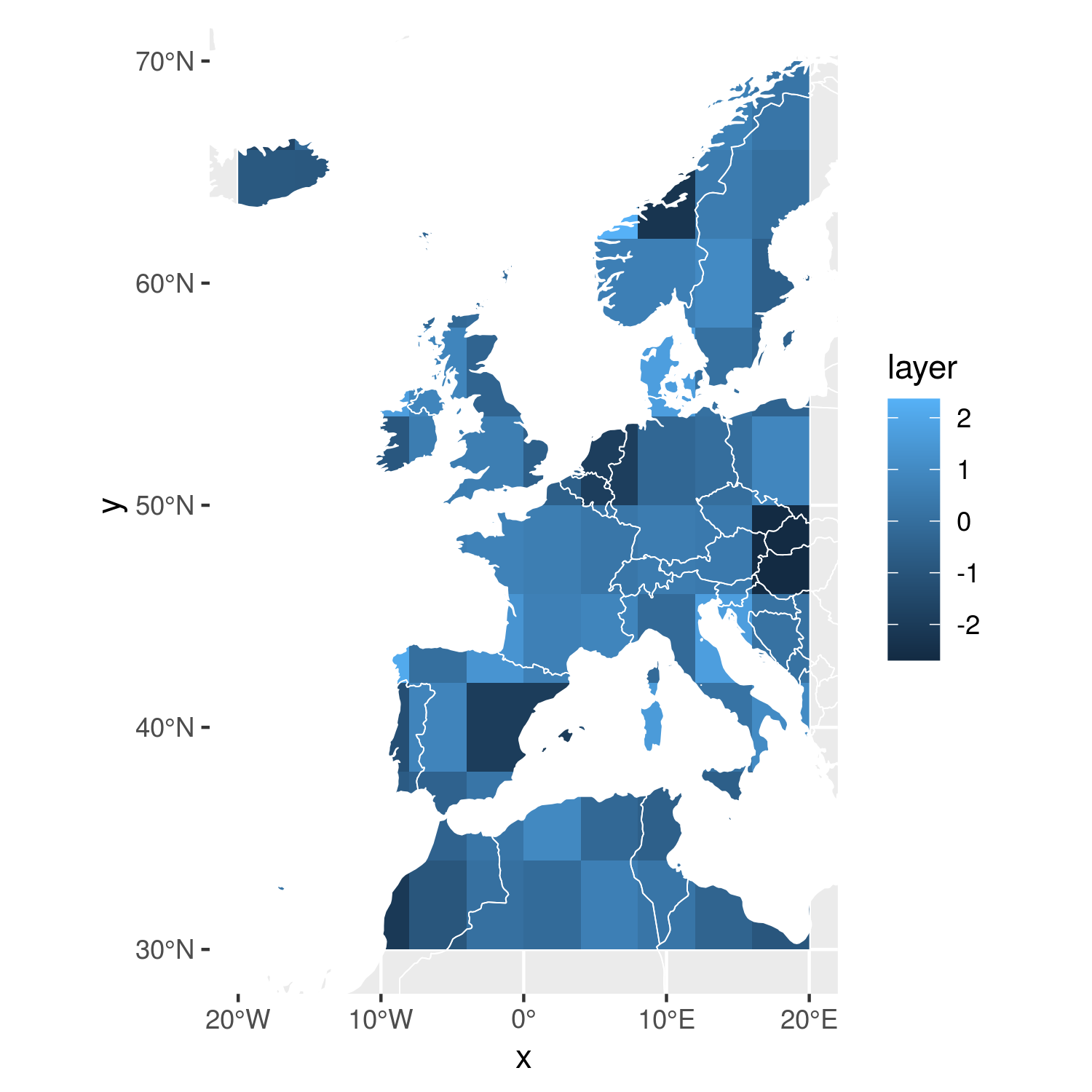
Upsampling
In order to work around this issue (in ggplot2) you can upsample the data using the raster package function disaggregate(), and subsequently mask using the desired vector polygon! Depending on the method used you can either smooth (set method to ‘bilinear’) or preserve the underlying coarse raster data in order to render a higher resolution plot masked to a specific polygon. The result is a subset of the original coarse resolution data with the fidelity of the vector data.
Unlike the previous method you create a lot of new raster data to work with. As such this method is rather memory intensive depending on the required output resolution. Be mindful of this when setting your upsampling parameters.
# UPSAMPLE 100x and mask, then
# convert to data frame
r_u <- disaggregate(r, 100)
r_u <- mask(r_u, countries)
r_u_df <- r_u %>%
  rasterToPoints %>%
  as.data.frame() %>%
  filter(layer!=0)

p <- ggplot() +
  geom_raster(data = r1_df,
            aes(x = x,
                y = y,
                fill = layer)) +
  scale_fill_continuous() +

  geom_sf(data = countries,
          color = "white",
          fill = NA,
          size = 0.2) +

  # crop the whole thing to size
  coord_sf(xlim = c(-20, 20),
           ylim = c(30, 70))

print(p)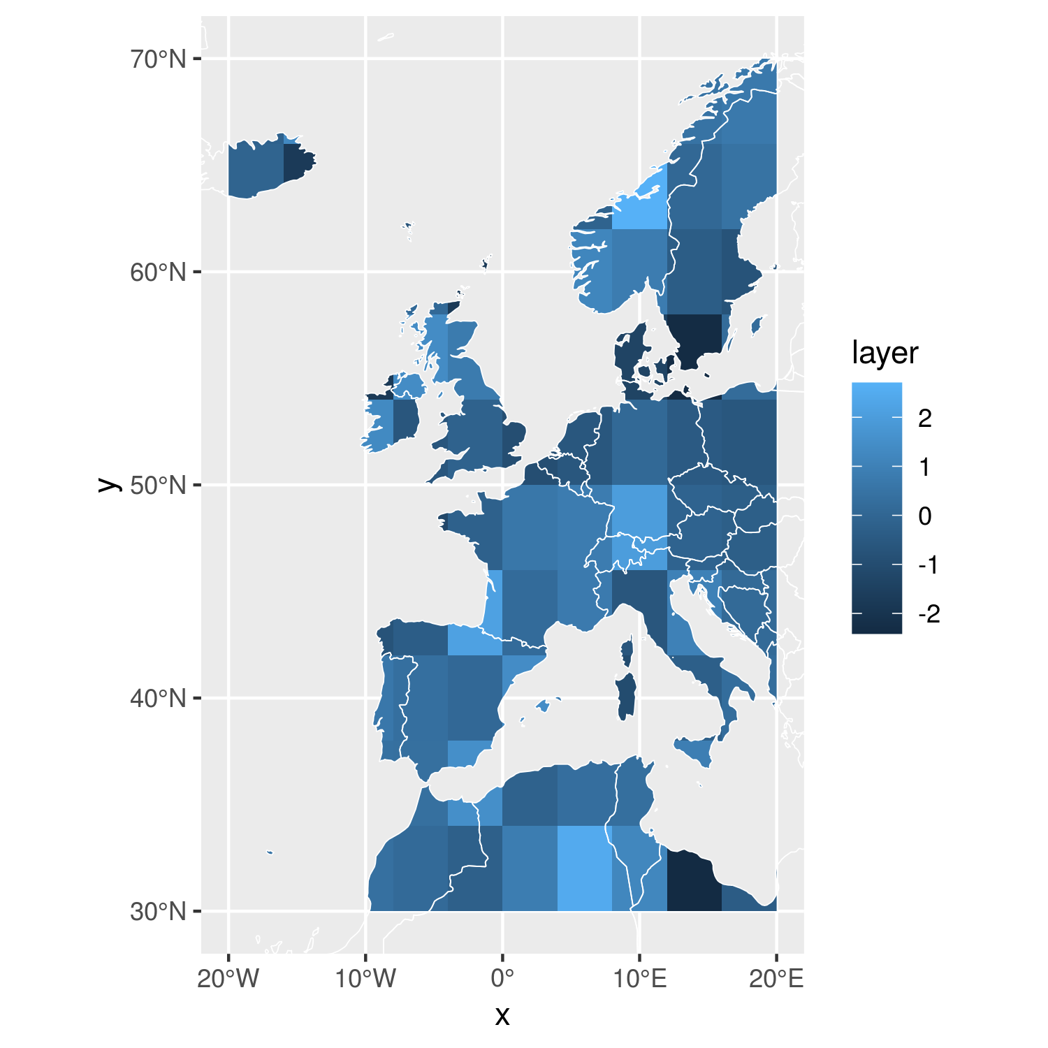
Wide borders
Finally, the last method is a variation on the cover up method. In some cases your data will cover your desired polygon almost perfectly, but the resolution of the plot and that of your data mismatches slightly (again providing “rough edges”). By over plotting with a wider polygon border you can cover up these imperfections, without having to download or provide additional masking polygons!
Final note, all these methods are (to some degree) resolution dependent, so be careful to check the output of your final renders when changing dimensions!
As always, keep an eye on our blog for new entries in this series on map building, and tips and tricks to improve your R mapping skills. The code for this project can be found on our github R tutorials page.